Dixon Coles and xG: together at last

In my previous post, I looked a little at the classic Dixon-Coles model and using an R package to experiment with it.

In this post, I’m going to look at a simple, flexible method that allows the standard Dixon-Coles model to incorporate expected goals (xG) data.

The Dixon-Coles model

The vanilla Dixon-Coles model is well documented online, and the original paper is also pretty approachable. I’d recommend spending some time getting acquainted with the model but I’ll run through some key features of the model here as well.

The core of the Dixon-Coles model is relatively simple. As with many sports, the goals scored per team per game are assumed to follow a Poisson distribution (I think Wikipedia’s explanation is actually pretty good here, and even includes a soccer example), with the mean (the predicted goals scored per game) for each team calculated by multiplying team offence and defence parameters like so:

where

The teams’ offence (α) and defence (β) parameters can then be estimated by maximum likelihood.

On top of this basic model, Dixon and Coles added two additional innovations.

The first is a parameter to control the correlation between home and away goals (“rho”, or ρ). In short, draws occur more often than you would expect by the model above. This is because teams’ goalscoring rates change depending on the scoreline and time remaining (amongst other things).

The second, which is relevant to what I’m discussing here, is to add a weighting of each game to the likelihood function. In the original paper, this is done in order to give more weight to recent games. In other words, it allows us to account for the fact that a 3-0 win yesterday affects our opinion of a team more than a 3-0 win a year ago.

Of course, the weighting function doesn’t just have to weight games based on when they occurred. We can weight games based on the competition (we care less about friendlies), or on the manager (we might want to downweight games under the previous coach), or even… xG?

What I’m going to do here is use this weighting function to allow the vanilla Dixon-Coles model to use per-shot expected goals value to estimate team strength and home advantage.

The data

But before we get to all that, we have to load the data. I’ve put the data required for this analysis up onto github, which you can download via the link below. It contains each shot and an accompanying expected goals value (xG) for the 2017/18 Premier League season.

library(tidyverse)

games <-
  read_csv("https://git.io/fNmRy") %>%
  filter(season == 2017) %>%
  nest(side, xg, .key = "shots")

# Preview data
head(games)

## # A tibble: 6 x 9
##   match_id date                home  away  hgoals agoals league season
##      <int> <dttm>              <chr> <chr>  <int>  <int> <chr>   <int>
## 1     7119 2017-08-11 19:45:00 Arse… Leic…      4      3 EPL      2017
## 2     7120 2017-08-12 12:30:00 Watf… Live…      3      3 EPL      2017
## 3     7121 2017-08-12 15:00:00 West… Bour…      1      0 EPL      2017
## 4     7122 2017-08-12 15:00:00 Sout… Swan…      0      0 EPL      2017
## 5     7123 2017-08-12 15:00:00 Chel… Burn…      2      3 EPL      2017
## 6     7124 2017-08-12 15:00:00 Crys… Hudd…      0      3 EPL      2017
## # ... with 1 more variable: shots <list>

Each row of the games dataframe contains a match, with each row of the shots column containing a dataframe of all of the shots in that game.

Preparing the data (simulation)

To incorporate the information expected goals tell us about team strengths, we need to put it into a form the Dixon-Coles model can work with: observed goals. We can do this via simulation.

We can think of each shot’s xG value as an estimate of it’s likelihood of resulting in a goal. A 0.2 xG shot corresponds to an estimated 20% chance of scoring. Using this, we can “replay” each shot of the match, randomly assigning a goal (or not) to each one, based on how good a chance it was.

We can do this, replaying each match over and over again to estimate each team’s performance based on the quality of the shots that they took. In our case, we want to get estimates of how likely each scoreline was.

Marek Kwiatowski points out that, using this method, each team’s goals will follow a Poisson-Binomial distribution. This means that we can estimate the scoreline probabilities analytically. Using the Poisson-Binomial distribution is also faster than Monte-Carlo simulation.

Handily, functions for working with the Poisson-Binomial distribution are available in the poisbinom R package, released to CRAN last year.

simulate_shots <- function(xgs) {
  tibble::tibble(goals = 0:length(xgs),
                 prob  = poisbinom::dpoisbinom(0:length(xgs), xgs))
}

simulate_game <- function(shot_xgs) {
  home_xgs <- shot_xgs %>% dplyr::filter(side == "h") %>% pull(xg)
  away_xgs <- shot_xgs %>% dplyr::filter(side == "a") %>% pull(xg)

  home_probs <- simulate_shots(home_xgs) %>% dplyr::rename_all(function(x) paste0("h", x))
  away_probs <- simulate_shots(away_xgs) %>% dplyr::rename_all(function(x) paste0("a", x))

  tidyr::crossing(home_probs, away_probs) %>%
    dplyr::mutate(prob = .data$hprob * .data$aprob)
}

simulated_games <-
  games %>%
  mutate(simulated_probabilities = map(shots, simulate_game)) %>%
  select(match_id, home, away, simulated_probabilities) %>%
  unnest(cols = c(simulated_probabilities)) %>%
  filter(prob > 0.001)  # Keep the number of rows vaguely reasonable

simulated_games

## # A tibble: 8,414 x 6
##    match_id home    away      hgoals agoals    prob
##       <int> <chr>   <chr>      <int>  <dbl>   <dbl>
##  1     7119 Arsenal Leicester      0      0 0.00548
##  2     7119 Arsenal Leicester      1      0 0.0211
##  3     7119 Arsenal Leicester      2      0 0.0340
##  4     7119 Arsenal Leicester      3      0 0.0307
##  5     7119 Arsenal Leicester      4      0 0.0175
##  6     7119 Arsenal Leicester      5      0 0.00679
##  7     7119 Arsenal Leicester      6      0 0.00188
##  8     7119 Arsenal Leicester      0      1 0.0187
##  9     7119 Arsenal Leicester      1      1 0.0718
## 10     7119 Arsenal Leicester      2      1 0.116
## # ... with 8,404 more rows

EDIT (2020-03-23): The above code has been updated to work with the latest version of the tidyr package after some breaking changes were included in the 1.0.0 release. Thanks to James Yorke and some folks on GitHub for pointing this out.

This can seem a little abstract, so let’s look quickly at a single game’s simulated results.

Each row of the resulting dataframe contains the estimated probability of a given scoreline in a given match:

example_simulation <-
  simulated_games %>%
  filter(home == "Arsenal",
         away == "Leicester") %>%
  arrange(hgoals + agoals)

head(example_simulation)

## # A tibble: 6 x 6
##   match_id home    away      hgoals agoals    prob
##      <int> <chr>   <chr>      <int>  <dbl>   <dbl>
## 1     7119 Arsenal Leicester      0      0 0.00548
## 2     7119 Arsenal Leicester      1      0 0.0211
## 3     7119 Arsenal Leicester      0      1 0.0187
## 4     7119 Arsenal Leicester      2      0 0.0340
## 5     7119 Arsenal Leicester      1      1 0.0718
## 6     7119 Arsenal Leicester      0      2 0.0179

So our 4-3 win has become a whole set of different possible scorelines, some more likely than others:

format_percent <- function(p) {
  rounded <- round(100 * p)
  ifelse(p < 0.01, "<1%", paste0(rounded, "%"))
}

example_simulation %>%
  ggplot(aes(x = hgoals, y = agoals)) +
  geom_tile(aes(alpha = prob), fill = "#08519c") +
  geom_label(aes(label = format_percent(prob),
                 colour = prob < 0.01)) +
  scale_alpha_continuous(range = c(0, 1)) +
  scale_colour_manual(values = c("black", "gray50")) +
  scale_x_continuous(breaks = 0:10, minor_breaks = NULL) +
  scale_y_continuous(breaks = 0:10, minor_breaks = NULL) +
  theme_minimal() +
  theme(panel.grid.major = element_line(linetype = "dotted"),
        legend.position = "none") +
  labs(title = "Simulated scoreline probabilities",
       subtitle = "Arsenal vs Leicester",
       x = "Home goals",
       y = "Away goals")

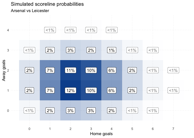
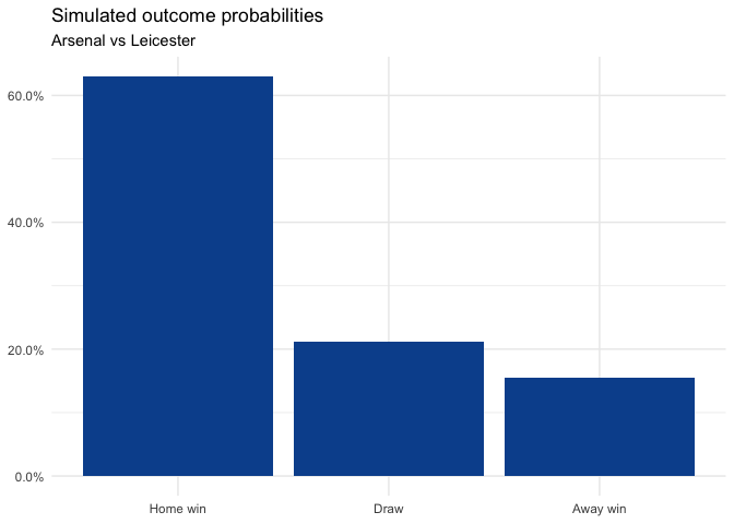
2-2 is the most likely scoreline given the shots taken; however, the overall match outcome is heavily in favour of Arsenal:

example_simulation %>%
  mutate(outcome = case_when(
    hgoals == agoals ~ "Draw",
    hgoals > agoals ~ "Home win",
    agoals > hgoals ~ "Away win"
  )) %>%
  count(outcome, wt = prob) %>%
  ggplot(aes(x = fct_rev(outcome), y = n)) +
  geom_col(fill = "#08519c") +
  scale_y_continuous(labels = scales::percent_format()) +
  theme_minimal() +
  labs(title = "Simulated outcome probabilities",
       subtitle = "Arsenal vs Leicester",
       x = NULL,
       y = NULL)

Fitting the model

The trick I’m introducing here is to feed these simulated scorelines into a Dixon-Coles model, weighting each one by its (simulated) probability of occurring. This allows us to “trick” the Dixon-Coles model, which uses actual goals, into using the extra information that xG contains about team strengths.

We can fit a Dixon-Coles model to the simulated scorelines and the actual scorelines using the regista R package, available via github.

# Uncomment and run the next line to install regista
# devtools::install_github("torvaney/regista")
library(regista)

# Fit a "vanilla" Dixon-Coles model (on observed goals)
fit_vanilla <- dixoncoles(
  hgoal = hgoals,
  agoal = agoals,
  hteam = home,
  ateam = away,
  data  = factor_teams(games, c("home", "away"))
)

# Fit on the simulated data, weighted by probability
fit_simulated <- dixoncoles(
  hgoal   = hgoals,
  agoal   = agoals,
  hteam   = home,
  ateam   = away,
  weights = prob,
  data    = factor_teams(simulated_games, c("home", "away"))
)

Estimating team strengths

We can then parse the team strength estimates into a dataframe to make them more pleasant to work with:

estimates <-
  inner_join(
    broom::tidy(fit_vanilla),
    broom::tidy(fit_simulated),
    by = c("parameter", "team"),
    suffix = c("_vanilla", "_xg")
  ) %>%
  mutate(value_vanilla = exp(value_vanilla),
         value_xg      = exp(value_xg))

# Preview results, ordered by the biggest difference
estimates %>%
  arrange(desc(abs(value_xg - value_vanilla))) %>%
  head()

## # A tibble: 6 x 4
##   parameter team              value_vanilla value_xg
##   <chr>     <chr>                     <dbl>    <dbl>
## 1 def       Manchester United         0.638    0.997
## 2 def       Burnley                   0.854    1.15
## 3 off       Crystal Palace            0.887    1.16
## 4 def       Leicester                 1.37     1.12
## 5 off       Manchester City           2.05     1.81
## 6 def       West Ham                  1.53     1.30

If we compare the vanilla estimates to the xG estimates we can see that they broadly agree, with the xG estimates being significantly more pessimistic about Burnley and Manchester United’s defence:

estimates %>%
  filter(!is.na(team)) %>%
  ggplot(aes(x = value_xg, y = value_vanilla)) +
  geom_abline(slope = 1, intercept = 0, linetype = "dotted") +
  geom_label(aes(label = team), size = 3) +
  scale_x_continuous(expand = expand_scale(mult = 0.3)) +
  facet_wrap(~ parameter, scales = "free") +
  labs(title = "Dixon-Coles parameter estimates",
       subtitle = "Based on ...",
       x = "... xG",
       y = "... goals")  +
  theme_bw() +
  theme(strip.background = element_rect(fill = "#9ecae1"))

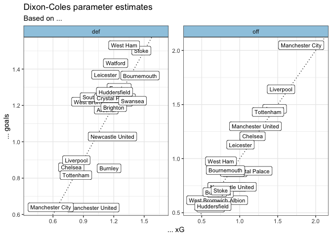
I don’t think these findings are controversial, and are simply a sign that the Dixon-Coles model is picking up on the information provided by each teams’ xG for and against. In any case, it is encouraging to see that this approach works.

Estimating home advantage

Pleasingly, the estimates for home advantage for both goals and expected goals come out to almost the exact same value:

estimates %>%
  filter(parameter == "hfa") %>%
  select(value_vanilla, value_xg)

## # A tibble: 1 x 2
##   value_vanilla value_xg
##           <dbl>    <dbl>
## 1          1.34     1.35

What about xG totals?

At this point you may be asking, “what does this approach give me that taking each team’s xG difference doesn’t?”. This is a good question to ask. I think there are a few important reasons for building a model like I have done here, but unless you’re interested in doing the modelling yourself, or making match predictions, I think xG difference will often be just as good.

I’ll go into why I think my approach is valuable, but first I want to show why xGD will do the job most of the time. We can see that over the course of a season, evaluating teams by xG for/against per game is more or less equivalent to the Dixon-Coles + xG approach:

sum_xg <- function(games, home_or_away) {
  # Helper function to sum the xG for and against in each team's `home_or_away`
  # games
  games %>%
    unnest() %>%
    count(!!home_or_away, side, wt = xg) %>%
    spread(side, n) %>%
    mutate(
      xgf = case_when(
        quo_name(home_or_away) == "home" ~ h,
        quo_name(home_or_away) == "away" ~ a
      ),
      xga = case_when(
        quo_name(home_or_away) == "away" ~ h,
        quo_name(home_or_away) == "home" ~ a
      )
    ) %>%
    select(team = !!home_or_away, xgf, xga)
}

# Compare to xG totals
xg_totals <-
  bind_rows(sum_xg(games, quo(home)),
            sum_xg(games, quo(away))) %>%
  group_by(team) %>%
  summarise(xgf = sum(xgf),
            xga = sum(xga))

method_comparison <-
  xg_totals %>%
    gather(parameter, value, -team) %>%
    mutate(parameter = case_when(
      parameter == "xgf" ~ "off",
      parameter == "xga" ~ "def"
    )) %>%
  inner_join(estimates, by = c("team", "parameter"))

method_comparison %>%
  ggplot(aes(x = value / 38, y = value_xg)) +
  geom_smooth(method = "lm") +
  geom_point() +
  facet_wrap(~ parameter, scales = "free") +
  labs(title = "Parameter estimate vs xG average",
       subtitle = "Each point represents one 2017/18 Premier League team",
       x = "xG per game",
       y = "Parameter estimate") +
  theme_bw() +
  theme(strip.background = element_rect(fill = "#9ecae1"))

So why bother with the Dixon-Coles approach at all?

The first reason is that the modelling approach I’ve outlined here gives us parameter estimates that can be combined to make predictions about football matches with no extra effort. Meanwhile, xG per game averages do not; if someone were to ask you how many goals per game a team averaging 1.2 xG for would score against a team conceding 1.2 xG, you’d have to build a model to work it out. Thankfully, no one in real life talks like that. But hopefully you see the point.

A second reason is that the model allows you to account for many other factors all at once. For the purposes of this post I’ve stuck to a simple formulation of the model, using offence, defence and home advantage. However, I can easily extend the Dixon-Coles-with-xG model to account for time discounting (giving more weight to recent games), friendlies, coach changes, …etc. Accounting for these factors all at once with raw xG tallies is much, much harder.

Likewise, by modelling the team strengths we get automatic adjustment for strength of schedule. Over the course of a full Premier League season this evens out (hence the clear line in the plot above). However, during the season being able to decompose xG tallies into team strength and schedule difficulty is useful.

A rule of thumb

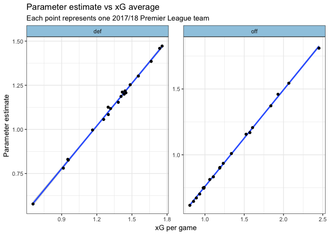
The plots above show a comically clear linear relationship between xG totals for/against and the parameter estimates. This means that it should be easy to go from one to the other.

As I mentioned above, one benefit of having parameter estimates is that it allows us to make predictions about matches. Therefore, by virtue of the linear relationship, we can create a rough rule of thumb to convert team xG totals ➡️ parameter estimates ➡️ match predictions:

linear_coeffs <-
  method_comparison %>%
  mutate(value_per_game = value / 38) %>%
  split(.$parameter) %>%
  map(~ lm(value_xg ~ value_per_game, data = .)) %>%
  map(pluck, "coefficients")

linear_coeffs

## $def
##    (Intercept) value_per_game
##     0.05249511     0.80589918
##
## $off
##    (Intercept) value_per_game
##     0.02657556     0.73339548

Therefore, with some rounding our rule of thumb to predict the goalscoring in a match between two teams becomes something like:

Other data and extensions

I’ve already explained how the model itself can be extended to estimate the effect of additional factors on match outcomes (or, I guess, xG generation), but I think the flexibility of this approach goes further than that. To use this method for adapting the Dixon-Coles model, you don’t necessarily need xG values at all. All you need is the probability of each scoreline occurring in each match.

With this in mind, the apprach could be used to infer team strength, home advantage, and anything else from a diverse set of ratings. One alternative to xG that I think would be particularly fruitful would be to use market odds to get the scoreline probabilities. The idea of extracting team ratings from betting odds is one I’ve found interesting in the past and I think this method would be effective as well.

Future work

This post is predicated on the assumption that using xG to estimate team strength is more accurate than goals alone. I think this is a fair assumption, but I would like to put it to the test, and compare the predictions made by our hybrid Dixon-Coles to the vanilla model. I think it will be interesting to see where and by how much the predictions differ.

In this post, I’ve presented a method for easily incorporating the information provided by xG into team strength estimates, while remaining flexible and extendible.