Predicting the Premier League with Dixon-Coles
In this post, I’m going to walk through one way of predicting the rest of the Premier League season with regista’s implementation of the Dixon-Coles model. I am going to demonstrate one method of using Monte Carlo simulation to predict various outcomes in the Premier League season.
In practice, this just means:
- Predicting the unplayed games,
- Sampling from those individual game predictions over and over again (“simulating” the rest of the season)
- Aggregate simulated games to get outcome probabilities
If the Dixon-Coles model is new to you, there are some previous explorations of the model on this site, and the original paper is very approachable.
Fetch the data
I’ll be using the data provided by football-data.co.uk.
To do this I have created a (very) minimal R package for downloading the data from the site, called footballdatr.
You can install it from github like so:
devtools::install_github("torvaney/footballdatr") |
It’s still very early, and so probably (definitely) has some bugs. If you do find anything, please don’t hesitate to let me know on twitter or on GitHub.
Nonetheless, we can use this to get the data for the 2018/19 English Premier League season.
library(tidyverse) |
## # A tibble: 200 x 23
##    competition date       home  away  hgoal agoal result hgoal_ht agoal_ht
##    <chr>       <date>     <fct> <fct> <int> <int> <chr>     <int>    <int>
##  1 E0          2018-08-10 Man … Leic…     2     1 H             1        0
##  2 E0          2018-08-11 Bour… Card…     2     0 H             1        0
##  3 E0          2018-08-11 Fulh… Crys…     0     2 A             0        1
##  4 E0          2018-08-11 Hudd… Chel…     0     3 A             0        2
##  5 E0          2018-08-11 Newc… Tott…     1     2 A             1        2
##  6 E0          2018-08-11 Watf… Brig…     2     0 H             1        0
##  7 E0          2018-08-11 Wolv… Ever…     2     2 D             1        1
##  8 E0          2018-08-12 Arse… Man …     0     2 A             0        1
##  9 E0          2018-08-12 Live… West…     4     0 H             2        0
## 10 E0          2018-08-12 Sout… Burn…     0     0 D             0        0
## # ... with 190 more rows, and 14 more variables: result_ht <chr>,
## #   hshot <int>, ashot <int>, hshot_on_target <int>,
## #   ashot_on_target <int>, hfoul <int>, afoul <int>, hcorner <int>,
## #   acorner <int>, hyellow <int>, ayellow <int>, hred <int>, ared <int>,
## #   closing_odds <list>
Predict the unplayed games
Work out the unplayed games
Fortunately, the Premier League’s schedule is relatively straightforward. Each team plays every other team at home and away. There are no playoffs, league splits or whatever they do in Belgium.
This means that we can find the unplayed games pretty easily. We can just take all combinations of teams, and filter out ones that have been played, or that feature a team playing itself.
teams <- factor(levels(data$home), levels = levels(data$home)) |
## # A tibble: 180 x 2
##    home        away
##    <fct>       <fct>
##  1 Man United  Watford
##  2 Man United  Liverpool
##  3 Man United  Southampton
##  4 Man United  Cardiff
##  5 Man United  Chelsea
##  6 Man United  West Ham
##  7 Man United  Brighton
##  8 Man United  Burnley
##  9 Man United  Man City
## 10 Bournemouth Fulham
## # ... with 170 more rows
Make predictions for those unplayed games
First, we have to fit a model that we can use to estimate how good each team is, and the effect of home advantage.
We can do this with regista’s implementation of the Dixon-Coles model. For the purposes of this post, we will just fit the model on the games played so far this season. However, a more comprehensive model may include matches from previous seasons, time-discounting, or even expected goals.
model <- dixoncoles(hgoal, agoal, home, away, data = data) |
##
## Dixon-Coles model with specification:
##
## Home goals: hgoal ~ off(home) + def(away) + hfa + 0
## Away goals: agoal ~ off(away) + def(home) + 0
## Weights   : 1
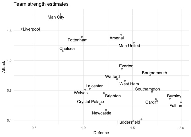
We can sense-check the model by looking at the team attack and defence parameters:
team_parameters <- |
It’s tempting to just calculate the match outcome (Home win/Draw/Away win) probabilities and go from there. It’s pretty easy to do with regista as well:
match_probabilities <- |
## # A tibble: 180 x 5
##    home        away        away_win  draw home_win
##    <fct>       <fct>          <dbl> <dbl>    <dbl>
##  1 Man United  Watford       0.232  0.220   0.549
##  2 Man United  Liverpool     0.770  0.165   0.0659
##  3 Man United  Southampton   0.124  0.166   0.710
##  4 Man United  Cardiff       0.0976 0.153   0.749
##  5 Man United  Chelsea       0.522  0.239   0.240
##  6 Man United  West Ham      0.208  0.209   0.582
##  7 Man United  Brighton      0.201  0.236   0.562
##  8 Man United  Burnley       0.0843 0.136   0.780
##  9 Man United  Man City      0.676  0.177   0.147
## 10 Bournemouth Fulham        0.152  0.206   0.642
## # ... with 170 more rows
This is enough to simulate match outcomes, and points scored. However, in cases where point totals at the end of the season are equal, we need goal-difference too.
Fortunately, this is something the Dixon-Coles model can handle. We can predict the probability of each scoreline for the unplayed games.
unplayed_scorelines <- |
## # A tibble: 19,563 x 5
##    home       away    hgoal agoal     prob
##    <fct>      <fct>   <int> <int>    <dbl>
##  1 Man United Watford     0     0 0.0348
##  2 Man United Watford     1     0 0.0468
##  3 Man United Watford     2     0 0.0634
##  4 Man United Watford     3     0 0.0475
##  5 Man United Watford     4     0 0.0267
##  6 Man United Watford     5     0 0.0120
##  7 Man United Watford     6     0 0.00448
##  8 Man United Watford     7     0 0.00144
##  9 Man United Watford     8     0 0.000404
## 10 Man United Watford     9     0 0.000101
## # ... with 19,553 more rows
Simulate the rest of the season
Join played game and unplayed games
There’s an added benefit to looking at the unplayed games like as scoreline-probabilities. We can look at the played games in exactly the same way. Any game that has already been played is simply a game where there is a single scoreline with 100% probability. This simplifies our simulation step, since we can treat both played and unplayed games the same.
played_scorelines <- |
## # A tibble: 19,763 x 5
##    home         away           hgoal agoal  prob
##    <fct>        <fct>          <int> <int> <dbl>
##  1 Man United   Leicester          2     1     1
##  2 Bournemouth  Cardiff            2     0     1
##  3 Fulham       Crystal Palace     0     2     1
##  4 Huddersfield Chelsea            0     3     1
##  5 Newcastle    Tottenham          1     2     1
##  6 Watford      Brighton           2     0     1
##  7 Wolves       Everton            2     2     1
##  8 Arsenal      Man City           0     2     1
##  9 Liverpool    West Ham           4     0     1
## 10 Southampton  Burnley            0     0     1
## # ... with 19,753 more rows
Simulate games by Monte Carlo
We can simulate the result of each game by picking a potential scoreline at random, where each pick is weighted by the estimated probability.
This gives us a single instance of a simulated season. We can repeat this over and over again to estimate the overall season probabilities. This is the Monte Carlo method of simulation.
simulate_season <- function(scoreline_probabilities) { |
## # A tibble: 5 x 5
##   home        away      hgoal agoal   prob
##   <fct>       <fct>     <int> <int>  <dbl>
## 1 Bournemouth Liverpool     0     4 1
## 2 West Ham    Arsenal       2     1 0.0610
## 3 Newcastle   Everton       0     2 0.0987
## 4 Liverpool   Watford       4     0 0.0959
## 5 Wolves      Liverpool     0     2 1
There are a few flawed assumptions being made in this simulation. I think it’s worth acknowledging a couple of them quickly:
- There’s no accounting for the possibility team-strengths changing
- From transfers
- From injuries
- Coaching changes
- etc
- There’s no accounting for motivation effects towards the end of the season
- Teams with nothing to play for are less likely to perform as well as others
These kinds of sources of model error should be considered when evaluating the model’s predictions, and when thinking about how you might improve the simulation method.
Calculating the league table
We care much more about overall table outcomes (Champion, Relegation, Top 4) than we do about individual results. So we need a way to calculate the table from a set of games:
calculate_table <- function(games) { |
We can check that this works as expected by checking the current table:
calculate_table(data) |
## # A tibble: 20 x 9
##    team               w     d     l    gf    ga    gd points position
##    <fct>          <int> <int> <int> <int> <int> <int>  <dbl>    <int>
##  1 Liverpool         17     3     0    48     8    40     54        1
##  2 Man City          15     2     3    54    16    38     47        2
##  3 Tottenham         15     0     5    43    21    22     45        3
##  4 Chelsea           13     4     3    38    16    22     43        4
##  5 Arsenal           11     5     4    42    30    12     38        5
##  6 Man United        10     5     5    41    32     9     35        6
##  7 Wolves             8     5     7    23    23     0     29        7
##  8 Leicester          8     4     8    24    23     1     28        8
##  9 Watford            8     4     8    27    28    -1     28        9
## 10 Everton            7     6     7    31    30     1     27       10
## 11 West Ham           8     3     9    27    30    -3     27       11
## 12 Bournemouth        8     2    10    28    37    -9     26       12
## 13 Brighton           7     4     9    22    27    -5     25       13
## 14 Crystal Palace     5     4    11    17    26    -9     19       14
## 15 Newcastle          4     6    10    15    27   -12     18       15
## 16 Cardiff            5     3    12    19    38   -19     18       16
## 17 Southampton        3     6    11    21    38   -17     15       17
## 18 Burnley            4     3    13    19    41   -22     15       18
## 19 Fulham             3     5    12    18    43   -25     14       19
## 20 Huddersfield       2     4    14    12    35   -23     10       20
Which also works on the simulated table:
calculate_table(single_simulation) |
## # A tibble: 20 x 9
##    team               w     d     l    gf    ga    gd points position
##    <fct>          <int> <int> <int> <int> <int> <int>  <dbl>    <int>
##  1 Liverpool         32     6     0   102    10    92    102        1
##  2 Man City          28     5     5    97    31    66     89        2
##  3 Tottenham         27     5     6    83    36    47     86        3
##  4 Chelsea           25     4     9    69    33    36     79        4
##  5 Arsenal           22     7     9    84    54    30     73        5
##  6 Man United        18     6    14    75    65    10     60        6
##  7 Everton           13    13    12    52    50     2     52        7
##  8 Leicester         14     9    15    41    47    -6     51        8
##  9 Wolves            14     7    17    41    43    -2     49        9
## 10 Bournemouth       12    10    16    55    65   -10     46       10
## 11 West Ham          13     7    18    52    62   -10     46       11
## 12 Brighton          12    10    16    40    51   -11     46       12
## 13 Cardiff           14     4    20    48    68   -20     46       13
## 14 Watford           12     9    17    48    56    -8     45       14
## 15 Newcastle         12     8    18    32    53   -21     44       15
## 16 Crystal Palace    10     9    19    31    51   -20     39       16
## 17 Southampton        9     9    20    42    71   -29     36       17
## 18 Fulham             7     7    24    32    86   -54     28       18
## 19 Burnley            6     8    24    30    78   -48     26       19
## 20 Huddersfield       4     9    25    24    68   -44     21       20
Running the simulations
Now we have everything we need to generate as many simulated league tables as we want.
n_simulations <- 1000 |
## # A tibble: 20,000 x 10
##    simulation_id team       w     d     l    gf    ga    gd points position
##    <chr>         <fct>  <int> <int> <int> <int> <int> <int>  <dbl>    <int>
##  1 1             Liver…    35     3     0    96    12    84    108        1
##  2 1             Man C…    27     6     5   101    32    69     87        2
##  3 1             Totte…    26     4     8    94    48    46     82        3
##  4 1             Chels…    21     9     8    67    31    36     72        4
##  5 1             Arsen…    22     5    11    82    61    21     71        5
##  6 1             Man U…    20     9     9    82    58    24     69        6
##  7 1             Leice…    18     8    12    52    43     9     62        7
##  8 1             Evert…    13    13    12    62    63    -1     52        8
##  9 1             Wolves    13    12    13    45    46    -1     51        9
## 10 1             West …    15     6    17    55    66   -11     51       10
## # ... with 19,990 more rows
Results
With the results in hand, we can move onto the fun parts. That is, sifting through our model’s predictions of the future.
Position probabilities
n_teams <- length(teams) |
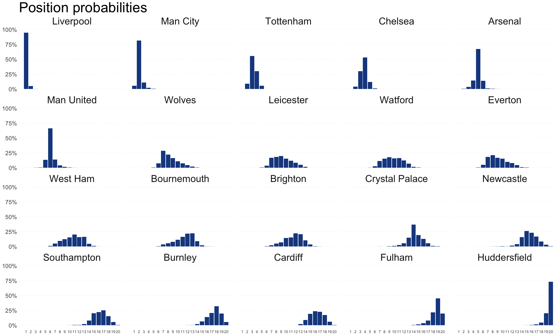
It turns out the model is extremely bullish on Liverpool’s chances of winning the league:
simulated_tables %>% |
## # A tibble: 2 x 2
##   team      p_win
##   <fct>     <dbl>
## 1 Liverpool 0.948
## 2 Man City  0.052
I think this is partly a reflection of the flaws in the simulation method. However, I think a bigger factor is using goals as our only input to team strength. As we know, the table does sometimes lie, and sometimes goals can deceive, too.
Both of these factors result in Liverpool’s chances being overestimated by the model. For comparison, the betting market has Liverpool at around 60% to win the league at the time of writing.
At the other end of the table, things are a bit more interesting; although Huddersfield and Fulham don’t look great.
simulated_tables %>% |
## # A tibble: 7 x 2
##   team           p_rel
##   <fct>          <dbl>
## 1 Huddersfield   0.981
## 2 Fulham         0.866
## 3 Burnley        0.569
## 4 Cardiff        0.24
## 5 Southampton    0.21
## 6 Newcastle      0.12
## 7 Crystal Palace 0.014
We can look at the race for the Champion’s League, too:
simulated_tables %>% |
## # A tibble: 5 x 2
##   team      p_top4
##   <fct>      <dbl>
## 1 Liverpool  1
## 2 Man City   0.998
## 3 Tottenham  0.944
## 4 Chelsea    0.872
## 5 Arsenal    0.178
Points totals
simulated_tables %>% |
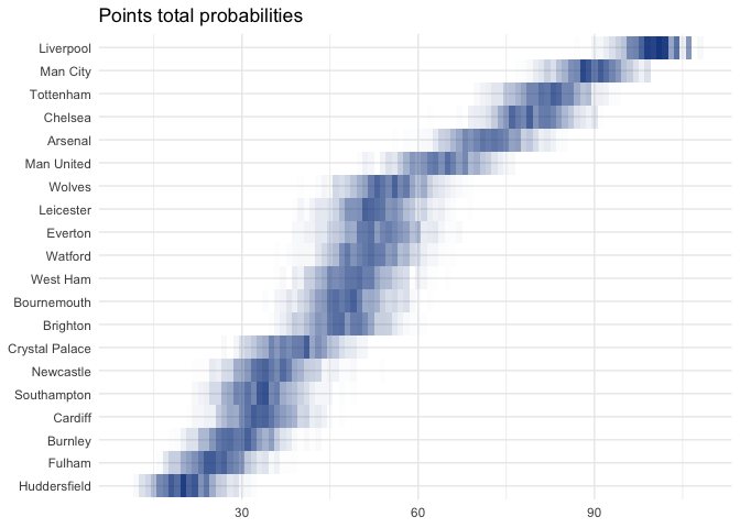
The model even seems to think that Liverpool’s chances of breaking 100 points are pretty good:
simulated_tables %>% |
## # A tibble: 1 x 2
##   team          p
##   <fct>     <dbl>
## 1 Liverpool 0.545
And even that they’ve got a solid chance of going unbeaten!
simulated_tables %>% |
## # A tibble: 1 x 2
##   team          p
##   <fct>     <dbl>
## 1 Liverpool 0.386
Wrap-up
This is one simple way of getting season-level predictions from a simple match-level model, using a relatively small amount of new code. Being able to quickly generate and investigate predictions is an important part of the data exploration process. Having both game and season-level views onto your model’s predictions, allows for increased insight into a model’s shortcomings and how it might be improved.
There are a few simple extensions to this analysis that could be nice jumping off points for improving the model.
- Time-discount factor
- What do the predictions look like if you incorporate more data from the past, with a time-discounting factor? (See the
weightsargument toregista::dixoncoles.)
- What do the predictions look like if you incorporate more data from the past, with a time-discounting factor? (See the
- Other leagues
- How does this analysis look when you try other leagues avaliable from football-data.co.uk? (Hint: change the first code chunk and try re-running the notebook)
- xG/Dixon-Coles
- How do the predictions look when you estimate team strength from xG rather than just goals? (See Dixon Coles and xG: together at last.)