What can time-discount rates tell us about xG and Goals?
Recently, I looked at backtesting and ensembling match prediction models. While working on this, I found a nice result regarding time discounting that I wanted to share.
What is time-discounting?
Match prediction models tend to produce estimates of teams’ attacking and defensive strength. The more accurate these estimates are, the more accurate the predictions. Factors like teams’ performance levels (or even home-field advantage) are dynamic and change over time. New players come into the team, team tactics are tweaked, and so on. Because of this dynamism, data (matches) from, say, a year ago tends to be less relevant than data from last week.
Time-discounting is a way of weighting input data in match prediction models such that more recent matches are given a higher weight (and therefore more influence on the model’s parameter estimates) than those in the distant past.
Signal vs staleness
If the most relevant information is data from the last week, the ideal scenario would be to use only the latest match for each team. But, we know that in practice that’s unlikely to work. A single match is quite noisy; anything can happen.
So to combat the noise in a single game, we have to add more data from further back in the past. But that historical data isn’t quite as relevant as the data from last week. How a team played a long time ago doesn’t tell us that much about the team’s performance level now.
So there’s a tension between having more data, and each incremental bit of data being progressively more out of date. Too much old data, and you’re feeding misleading information into the model. Not enough data, and the model can’t separate the signal from the noise.
More signal = less data
If we use data that has less noise, we don’t have to use as much to extract a reliable signal. So instead of using more data, we can try to use better data.
This is broadly the logic of using expected goals (xG) instead of goals to evaluate teams and players. Goals are really noisy, so over the course of a season, there is still more signal in xG. To reliably evaluate teams on goals with the same confidence, you’d need years of data, at which point the coach has changed, the squad has changed… you’re comparing multiple different teams!
Exponential weighting
The most common form[1] of time-discount is exponential weighting, where each data point is weighted according to the formula:
where “
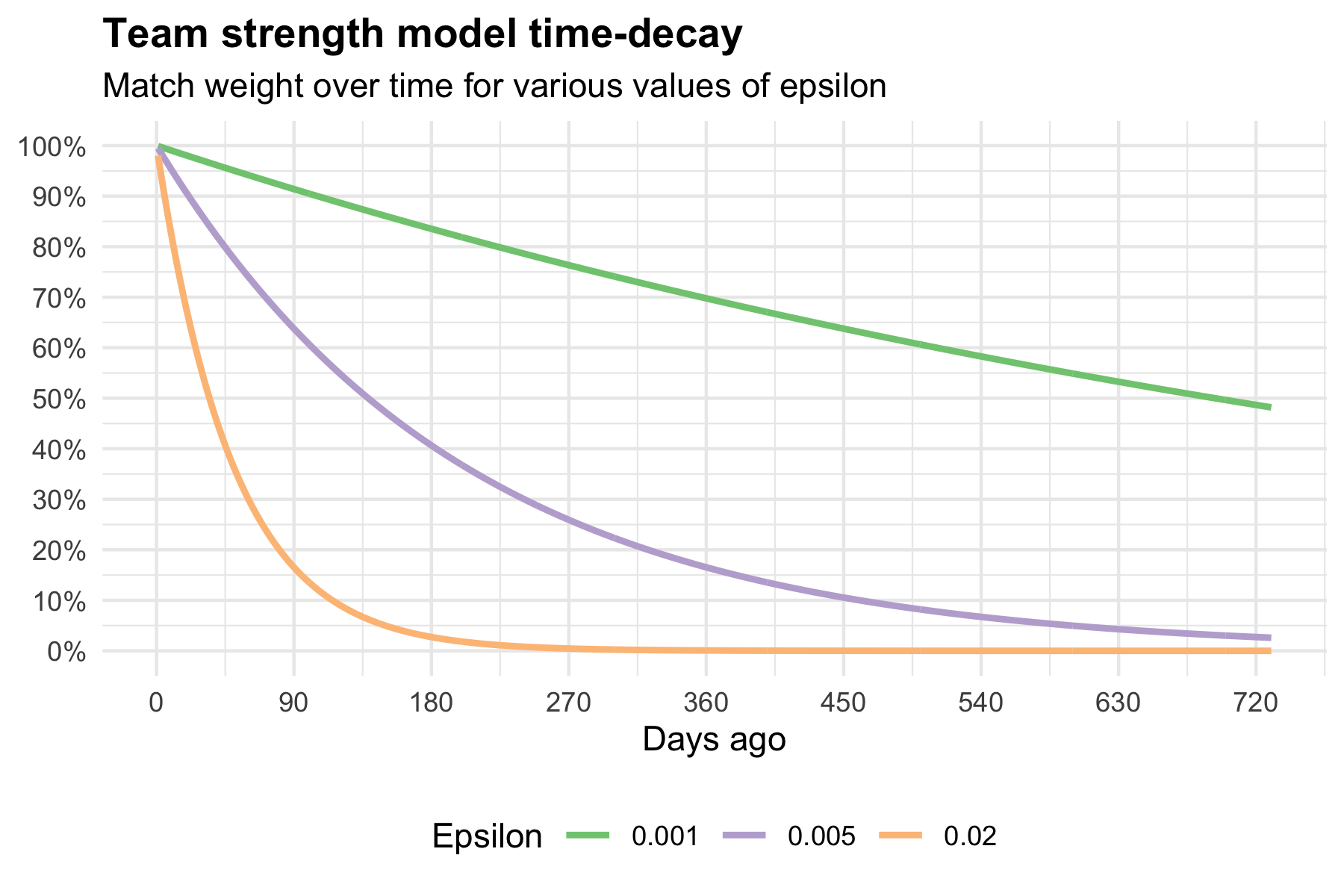
Because of the nature of exponential decay, a high discount rate (yellow line) results in a very low weight for matches a long time in the past compared to a low discount rate (green line).
How do you find the right value of “
The simplest solution is to use backtesting. In short, this means training the model for a variety of different values of epsilon and seeing which one results in the best predictions.
Time-discounting with different models
If we backtest both Goals-based and xG-based models for a variety of “
On the x-axis, I have plotted the weight at day 365 (

Both plots show the same overall shape: a very low weight at day 365 (i.e. a very high discount weight), leads to very poor performance followed by a sharp rise, a peak, and a slower decline as the discount rate increases (and old data is given more importance).
The peak model performance for the xG-based model comes at with a weight at day 365 of around 25%. On the other hand, the peak performance for the goals-based model comes at around 50% weight-at-day-365.
This goes back to what I mentioned earlier about signal-vs-noise. A goal-based model needs to give matches from the past a higher weight because goals are a noisy data source. Whereas the xG-based model performs best with a higher discount rate, because it’s able to extract more information from each match. Or, to put it another way, it requires less information before the staleness of additional data-points starts to harm the model’s performance.
We already knew xG was a better way to evaluate teams both intuitively and empirically, but I think looking at the comparison of goals and xG through the time-discounting is a nice way to develop our intuition about why xG is better.
Appendix I: A more entrenched elite?
EDIT (2020-07-19): Originally, I speculated that a change in “
Thanks to Diogo for pointing this out to me on Twitter.
Original text (click to expand)
As a final note, the original Dixon-Coles paper from 1997, they estimate an optimal value of “
Assuming I’ve correctly reproduced their method, what might be the cause of this change? Could it be that a more entrenched elite at the top of the Premier League has meant that old (e.g. 6+ months ago) results have more information about the present?
We talk a lot about how the economics of the game have changed and made it harder for small clubs to compete, so I think this is an interesting hypothesis. Especially as this could give us an empirical way to measure those changes. I don’t think we can evaluate from this analysis alone whether it this is driving the change in “
Appendix II: Code etc
If you would like to reproduce this analysis, or dig a bit more into the technical details, the code can be found in my wingback (because it’s concerned with back-testing models… I couldn’t help myself, I’m sorry) repository.
This repo is built on top of understat-db, a project for pulling data from Understat.com into a database. It uses a Python library called mezzala for modelling team-strengths and match predictions.
Appendix III: Data scarves
I still have some Liverpool 2019/20 “data scarves” left for sale (shipping to the UK). If football+data is your thing, take a look:

The most common form that I know of. If you know of any others that you think might work better, let me know! I’d love to try them out. ↩︎