Should we stop using moving averages?
Recently, I’ve seen a few posts looking at rolling averages for some team and player metrics. I think that rolling averages have some flaws. Maybe exponentially-weighted averages are a bit better?
What is bad about moving averages?
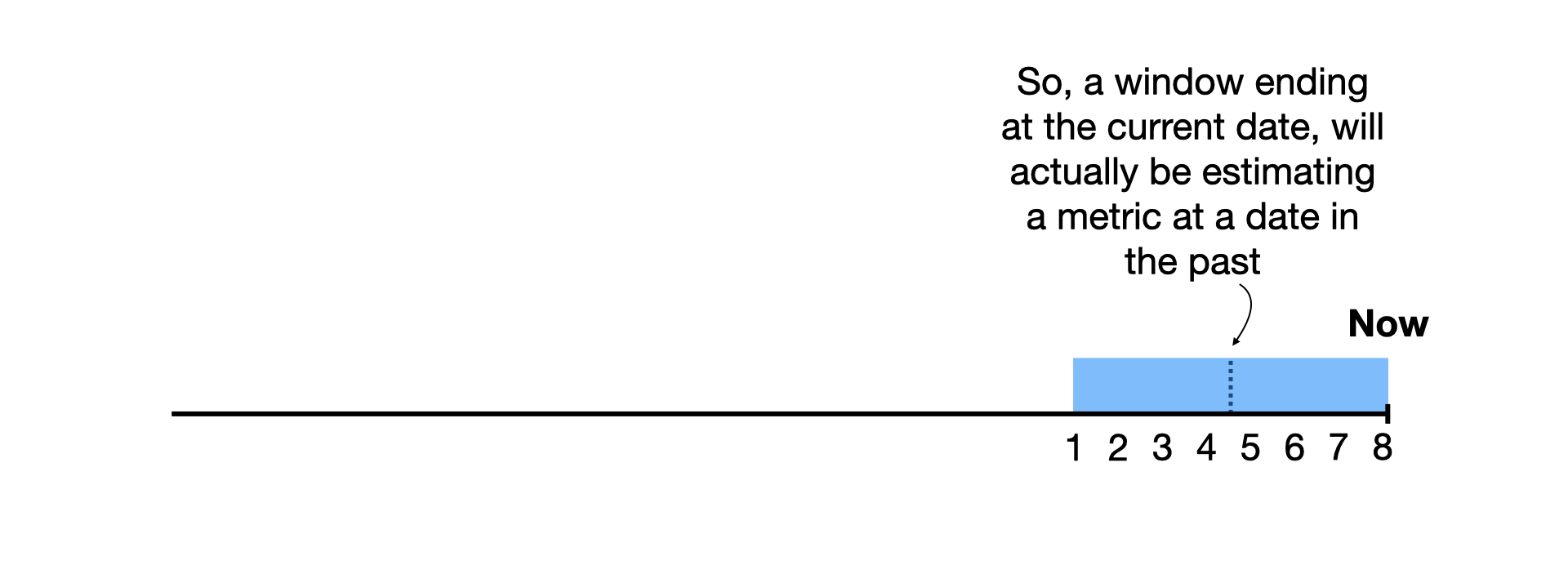
In short, when taking a moving average of a given metric, you end up estimating that metric for a date in the past.
Let me explain:
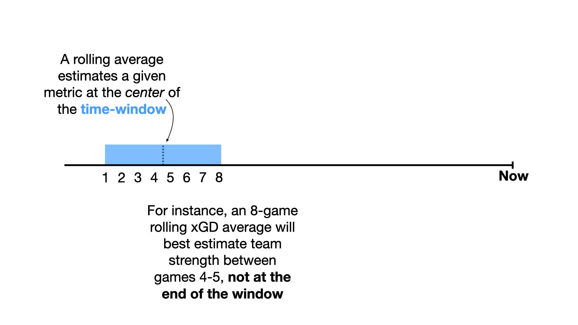
So, when using a rolling average, the time window should enclose the date of interest, not end at the date of interest.
However, this presents a problem when the date of interest is close to the current date:
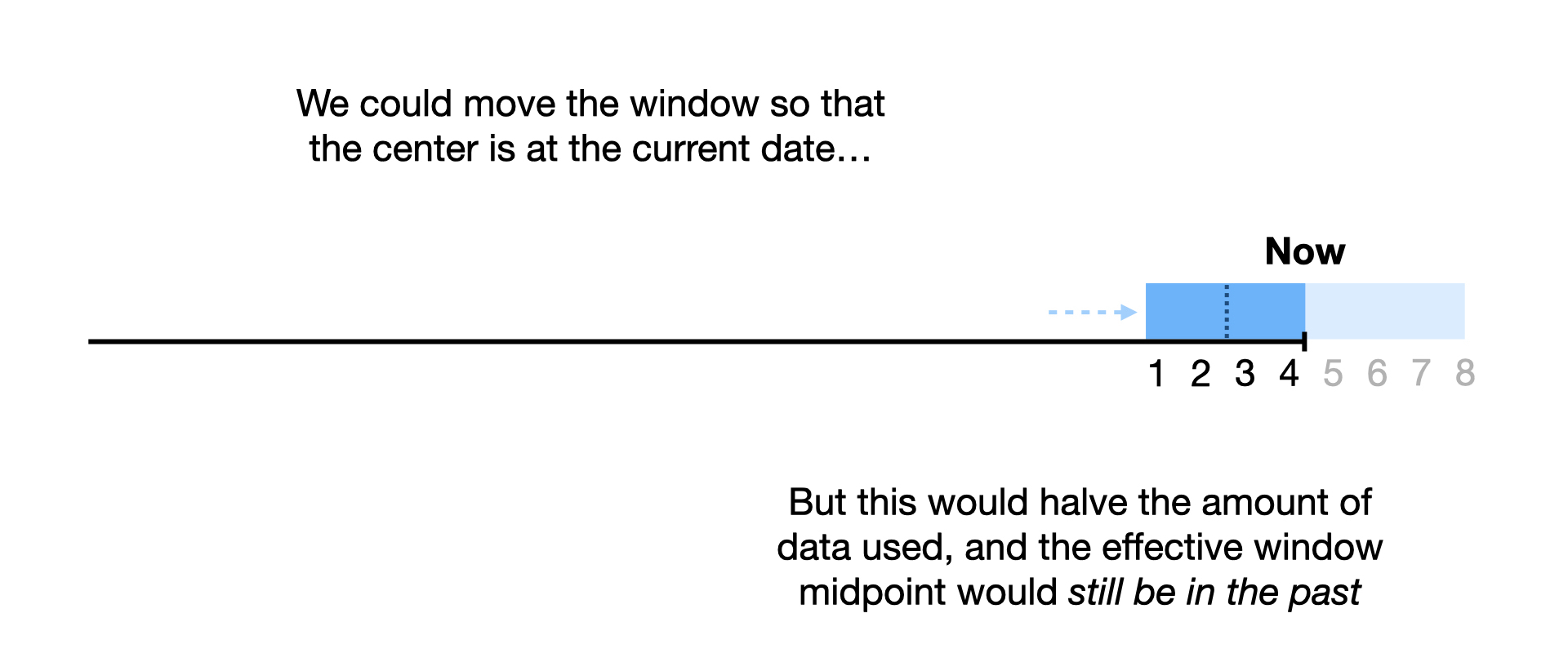
What can we do to fix this?
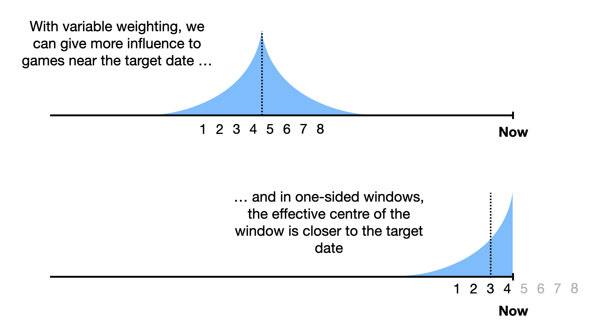
Part of the problem is that all games within the window are given an equal weighting. To shift the center of the window towards the date of interest, matches close to that date should be given a higher weighting than those far away.
Once we start looking at this as a weighted average, I think it is a little more intuitive to weight things in this manner than it is to assign games a weight of either 0.0 or 1.0 depending on whether they fall into the time window.
So what exactly should this weighting look like?
Recently, I’ve been interested in how modelling can inform simpler, more heuristic approaches. In this case, I think we can learn from the time-discounting methods that are used in modelling football teams’ strength.
Team strength models share a goal with moving averages: estimating something at a given date. The most common approach I have seen for weighting input data in team-strength models is an exponential weighted average:
where “
If we applied this to replace a moving average, the weighting would look something like this:
Note that with an exponentially decaying weight, the weight will never drop down to zero. In practice, picking a cutoff beyond which games aren’t included might be useful. This cutoff could be in the form of a time window (e.g. 6 months from the target date) or in the form of a minimum weight (e.g. “games where weight >= 0.01”)
So, what difference does it make?
For no particular reason, let’s look at the rolling non-penalty xGD of Manchester United:
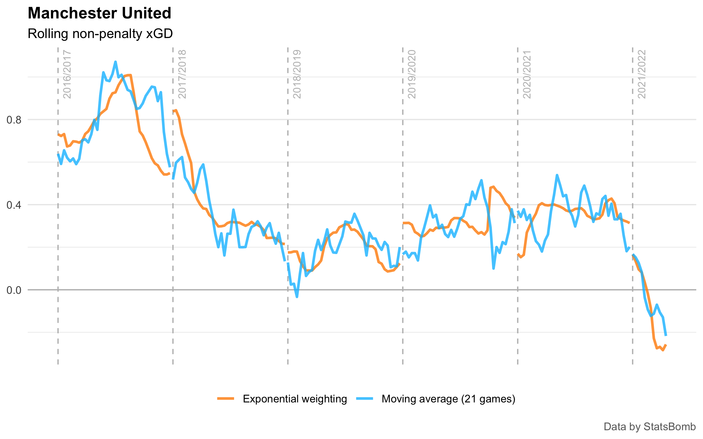
Here, the blue line shows a 21-game moving average, centered on the match of interest. In other words, for each match, we take the 10 matches before and the 10 matches after, and construct an average.
The orange line shows the exponentially-weighted moving average. Here, I used an “
In both cases, the moving averages use both past and future data where available. I haven’t shown the uncentered “last 20 games” style of moving average, since it is almost identical to the blue line but shunted 10 games to the right.
Although the overall shape of the curves is the same, there are 2 main differences between the 2 moving averages shown above.
The main difference is that the exponential weighting gives a smoother curve. This is because games in the past have incrementally less influence on the average, instead of going from being given equal weight to being not included at all.
I’m not entirely sure how many sharp changes we should expect to see in an abstract quantity like team ability (that xGD is serving as an indicator for). In general, I would guess that changes should be smooth, but I can see how things like player injuries and coach changes, for example, could reasonably cause discontinuities. However, I don’t trust that the sharp peaks and troughs we see in the moving average are anything other than noise. The whole point of a moving average is to smooth out the noise to more clearly indicate trends, and I think it’s reasonable to say that the exponential weighting is doing this a bit better.
The other difference we can see in this chart is that the exponential curve has much bigger jumps at the start/end of each season. This is because I calculated the weighting on the basis of time rather than on the basis of “how many matches ago”. At the start of the season, the matches from the end of last season took place a reasonably long time ago, so the current-season games have much more influence on the weighted average.
You could argue this makes for a slightly unfair comparison between the methods. Perhaps using a weighting function where “
The biggest individual difference between the two methods can be seen towards the end of the 2019/20 season.
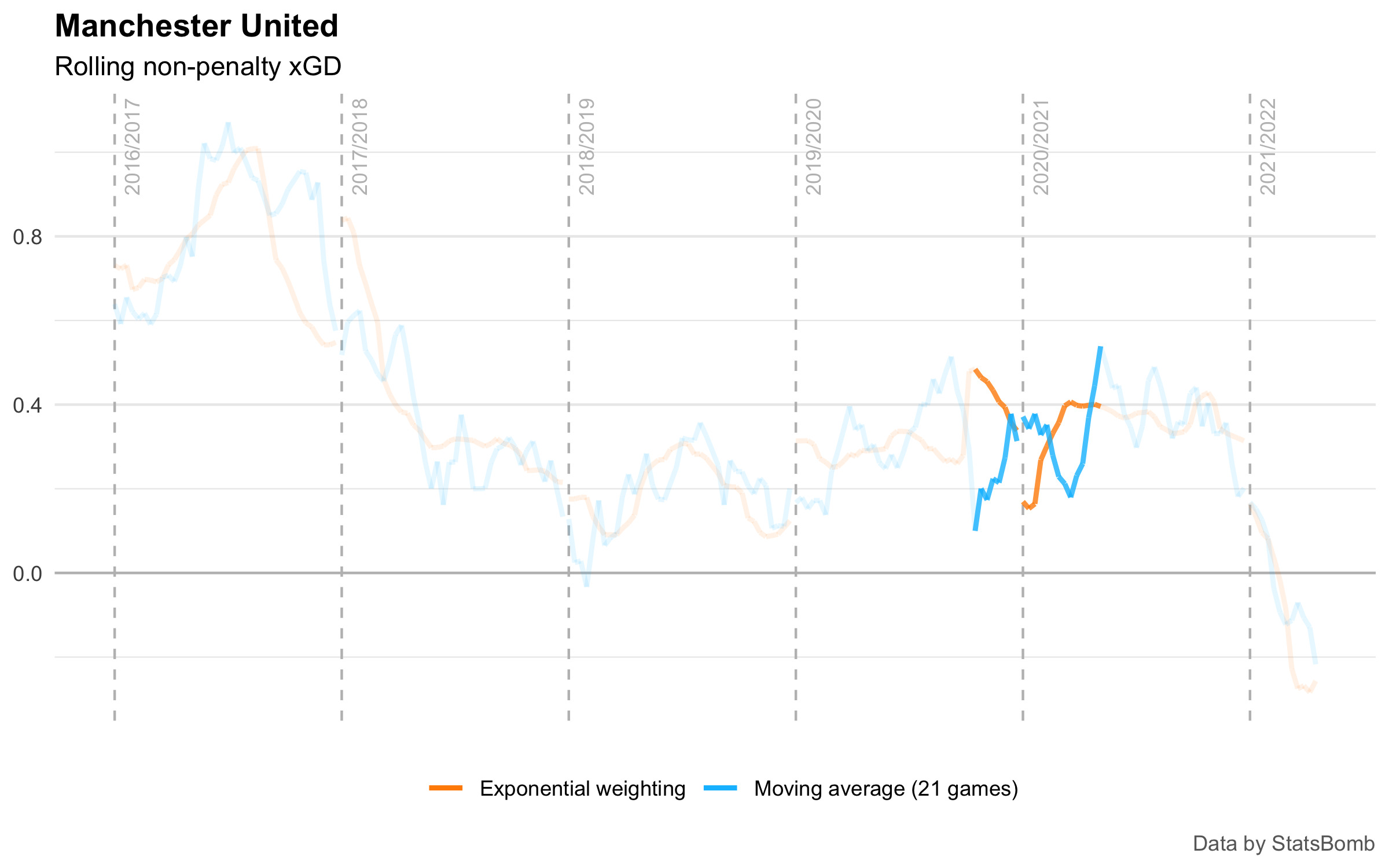
In this case, the moving average shifts to include two games from 2020/21 with large negative xGD tallies:
- Brighton 1.56 - 0.27 Manchester United
- Manchester United 0.16 - 2.91 Tottenham Hotspur
This results in the moving average sharply dropping down.
However, because those matches take place next season, and because of the Covid-induced mid-season break lowering the weight of earlier games, the exponentially-weighted average gives more influence to the stronger performances at the end of 2019/20.
I don’t think either of these approaches can be considered “correct” in any meaningful sense. But I do think that the exponentially-weighted average better reflects the performances of the team at the time in question. How much should our opinion of Manchester United at the end of 2019/20 be affected by a thrashing at the start of 2020/21? Probably a bit, but not as much as performances in 2019/20.
Not just team metrics
This approach doesn’t have to be restricted to just team-level metrics. We can easily apply the same logic to player stats.
Take Harry Kane’s xG scored from open play p90:
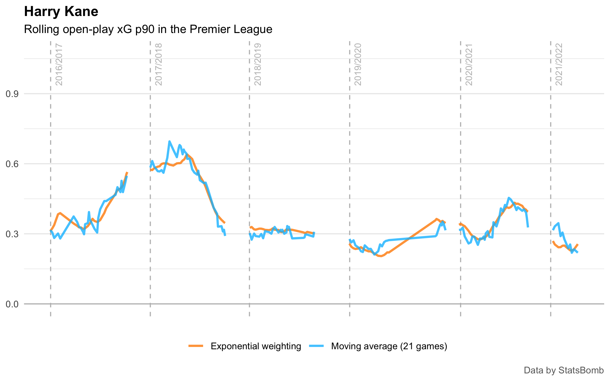
Again, the shape is basically the same, but the smoothing has improved.
Conclusion
I’ve suggested 3 changes to try and make rolling-averages better:
- Center the average on the date of interest, instead of using the last n games (or similar)
- Use an (exponential) weighting instead of a moving window
- Calculate weighting using time instead of match index (“how many matches ago”)
Ultimately, if you follow the logic of improving a moving average far enough, you’ll end up at statistical modelling. But this is a step up in complexity and is often harder to explain than a weighted average. An approach like this can yield some improvement without too much additional complexity.
It’s a little more work, but maybe it’s worth it?
What do you think?